Easy Spatial Alignment of ICEYE SAR Data for Machine Learning

After the release of the icecube toolkit, we decided to develop a dockerized Sentinel Application Platform (SNAP) coregistration routine to reduce the burden of spatially aligning a stack of time-series synthetic aperture radar (SAR) images and facilitate SAR-based machine learning.

This is our third blog about machine learning (ML). It was first published on Medium and is one of a five-part series in the AI4SAR project. AI4SAR is an ESA Φ-lab sponsored project with the objective to lower the entry barrier for SAR-based ML applications. If you haven’t heard about it yet, visit our project page!

Our first ML blog covers machine learning for SAR images and discusses ICEYE’s focus in the AI4SAR project and the second blog discusses the icecube toolkit for creating datacubes for supervised ML using ICEYE SAR images. 

In this blog, you will discover how to coregister ICEYE images using SNAP without the burden to set up your environment and install additional software. At the end of this blog, you will learn how to create a georeferenced product with a single line of code.

What Is Coregistration?

Coregistration, the spatial alignment of images, is a time-consuming but foundational pre-processing step that you must perform when you work with time-series stacks of SAR images. It ensures that features in one image overlap with those in the other images that will be stacked together.

Precise coregistration of SAR images is a nontrivial task because a change in the acquisition geometry generates image shifts that, in principle, depend on the topography.

To illustrate this shift, let’s use two images from a dataset that we released to give our community the opportunity to test the icecube toolkit with a real dataset. Image ID 71820 is the primary or baseline image and image ID 73908 is the secondary image. If you try to overlay the different rasters on top of each other, you will observe some interesting effects.

For example, if you build a two-band composite where the first layer is the primary image (green channel) and the second layer is the secondary image (red channel), you will notice a 3D effect around the edges. This effect indicates that the primary image is not aligned with the secondary image.

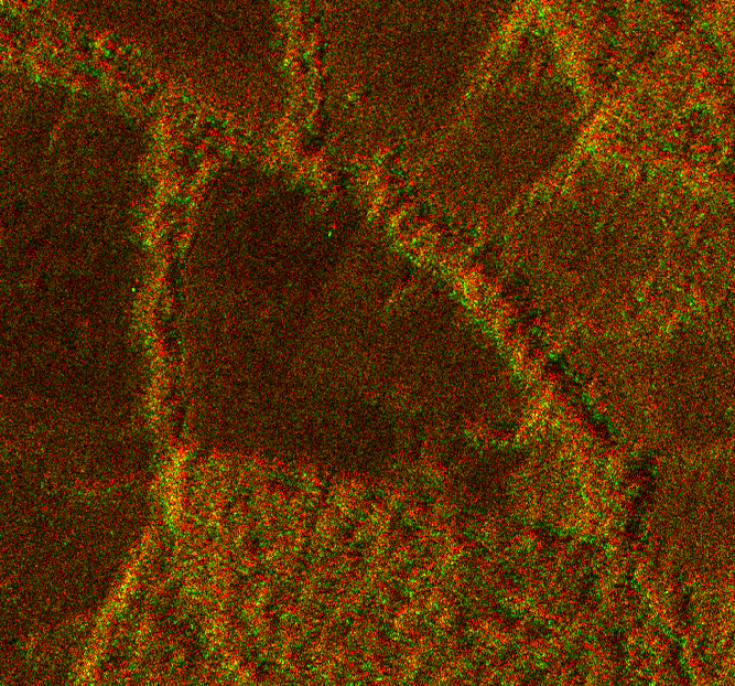
Figure 1. 3D effects occur at the edges of surface structures when you overlay two images without prior spatial alignment. Green marks the edges in the first image and red the edges in the second image.

After coregistration, the edges match and the new composite image from the primary image (green channel) and the secondary, coregistered image (red channel) is clear.

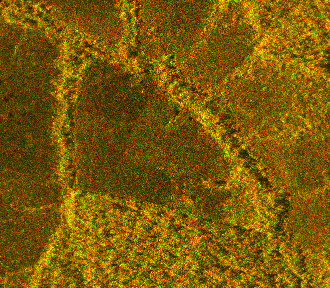
Figure 2. Sharp edges stand out after the two images are spatially aligned.

The two image examples demonstrate how important coregistration is for a time-series analysis. Even a slight shift of a few meters between two rasters can ruin your analysis, because the pixels do not represent the same object on the ground.

Generally speaking, coregistration requires the identification of common features like road junctions or river crossings in the primary image and the warping of the other images to match the common features of the primary image.

SNAP FOR ICEYE IMAGERY

SNAP is an open-source, common architecture for all ESA toolboxes that is ideal for the exploitation of Earth Observation (EO) data. While SNAP is primarily used to manipulate Sentinel data, you can use it for ICEYE data as well.

Developing a layer on top of SNAP to coregister ICEYE images was a natural progression of our ongoing effort to leverage the existing open-source tools and strengthen our collaboration with ESA Φ-lab. But why are we dockerizing the solution if you can download SNAP and run the coregistration function from its UI?

We are aware that not all icecube users/ML practitioners are familiar with remote sensing products and pre-processing steps, such as coregistration. To lower the entry barrier - the primary motivation for the AI4SAR project -  we want to reduce the number of operations that need to be performed before getting started with the icecube toolkit. 

Therefore, we offer an end-to-end solution. The dockerized routine includes a module that maps the metadata of the coregistered images to comply with the ICEYE product guidelines. This way, our users don't have to bother with the intricacies of dealing with proprietary data. Finally, we would like to enable the coregistration step to be integrated into different pipelines, which can be easily achieved via a command line interface (CLI).

You can use any method to coregister the images. You will always be able to use them with the icecube toolkit. The idea with this dockerized routine is to open source the complete processing chain (coregistration -> stacking -> tiling) so that anyone can analyze the ICEYE time-series data (and you have a free dataset to play with!)

Now let's take a look at what's happening behind the scenes.

The docker uses the SNAP 8.0 graph builder to coregister two images. Users can choose one of the three methods to coregister these images (dem_assisted, cross-correlation, and create stack). These are represented by three different SNAP execution graphs inside the docker.

When the coregistration is done, a metadata wrapper assigns the correct metadata to the coregistered images. Figure 3 illustrates this process.

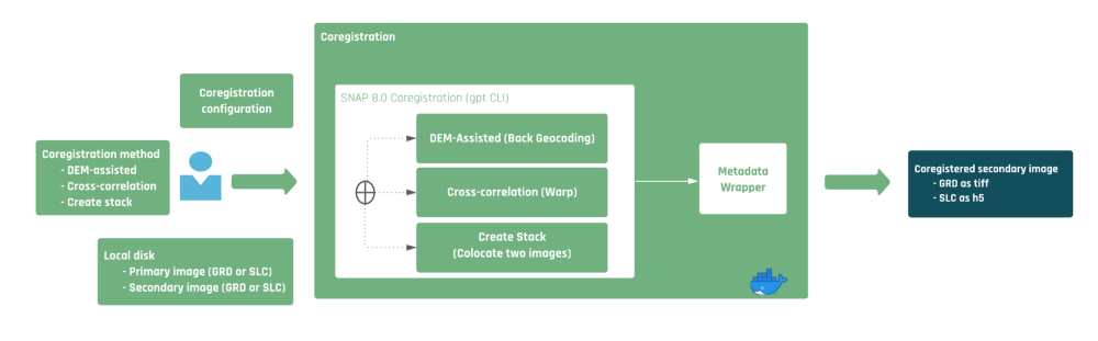
Figure 3. Workflow of the dockerized coregistration process, including the georeferenced output that you can load into the icecube toolkit or your geospatial application of choice.

Let’s Coregister Two Images

Perform the following steps to coregister two images:

DEM-assisted is the default coregistration method. For more information on this method, see this IEEE journal paper.

1. Download the publicly available dataset comprising four ICEYE images taken within 12 days.

2. Select any two GRD images from the dataset and move them to one folder. For example, ICEYE_GRD_SM_71820_20210722T055012 and ICEYE_GRD_SM_73908_20210727T055021.

3. Pull the snap_coregister image from dockerHub. The docker image requires 16GB of RAM (Change the image tag from latest to gpt27go if you have 32GB of RAM).

4. Type the following commands to coregister the GRD images.

5. (Optional) Use coregistration_type to change the default coregistration method. You can set it to cross-correlation or create stack. Additionally, you can use config_path (local file path) to edit the config.yaml file that contains the parameters associated with each method.

Here are the default parameters for each coregistration method.

For more information on each parameter, see the SNAP help content.

(GRD and SLC) For the DEM-assisted method, you can modify the following parameters:

(GRD) For the cross-correlation method, you can modify the following parameters:

(SLC) For the cross-correlation method, you can modify the following parameters:

Build Your First ICEcube

The dockerized SNAP coregistration routine helps you get a georeferenced output with just a single line of code without installing additional dependencies. However, it is important to note that the routine is a wrapper around SNAP. It simplifies the process, but does not replace SNAP.

If this blog piqued your interest, jump right to this detailed notebook to build your first ICEcube now!